Introduction
This is a guide to identifying how people answered questions asked by the British Election Study, over time, using R. I wrote this guide because I could not find a pre-existing one. It has been cobbled together from multiple helpful blogs and teaching tools, and some direct help from Professor Chris Hanretty. You can find these sources via links in the Acknowledgements. They ensured my code was functional, and its flaws are not their fault.
The data and code is compiled in this zip file but you can also download the surveys separately.
Why should I care?
Combining annual surveys to visualise how responses to the same question change over time is a fundamental part of modern political science. As one of the oldest continuous British political surveys, the BES is often used to visualize cross-time changes in attitudes. For example, Fieldhouse et al.’s 2019 book Electoral Shocks used it to show the decline of partisanship in Britain since the 1960s. Other studies, such as Ford & Sobolewska’s Brexitland, use the British Social Attitudes Survey for much the same purpose.
Despite this widespread use, there seems to be no readily accessible guide to performing such combinations using free software. Everyone who wants to do this must therefore learn for themselves. This increases the opportunity cost for performing analysis. Providing some copy-pasteable code reduces that opportunity cost, and hopefully makes this vital tool of political analysis just a little bit more accessible.
1) Obtaining R, R Studio, necessary R packages and the BES data.
To download R, and the ever-useful interface R Studio, I recommend following the guide available at https://socviz.co/index.html#preface
This preface also provides (down at the very bottom) instructions on how to download R packages. You need to have these packages installed for the commands below to work. In this guide we will be using the packages tidyverse, haven, survey, srvyr, and here.
To activate these packages you use the library command, as shown below:
library(tidyverse)
Remember, you must reactivate each package every time you open R Studio.
The BES data is available for download from https://www.britishelectionstudy.com/data-objects/cross-sectional-data/
To gain access to it, you will need to make a free account on the BES website. I recommend downloading the STATA files, and all the associated PDFs and Word Documents. You will need the latter to find out the questions these surveys ask.
2) Input the BES data into R.
We start by getting the BES data into R. The first step is to tell R where it should find the BES data, by setting the ‘working directory’. Happily, we do not need any code to do this. If we open our R session using an R Project file (eg. one with the .Rproj extension), R automatically makes the folder that .Rproj file is in the working directory. For the following code to work then, make sure:
- You open R by double-clicking a .Rproj file.
- That that .Rproj file is located in the same folder as your data files.
If you do not already have an .Rproj file in the same folder, you must create one. This instructional video will show you how to make your R session into a project: https://www.youtube.com/watch?v=etkSsF6r2iU&ab_channel=LockeDataLtd.
If you would prefer to organise your data more neatly (eg. so that everything is not in one big folder) I provide links to some useful blog posts in the Acknowledgements section at the end of the blog.
Now to input the data!
To input the data, we use the read_dta command from the haven package. For example:
bes1987 <- read_dta(here("bes1987.dta"))
This tells R which file to read in. Be careful to write the exact name of the file you want in between the quotation marks. If the command doesn’t work, the first thing you should do is check for misspellings.
3) Determining which variables you want to examine
The BES does not ask the same questions every year.
To find out how many of the BES surveys ask the question you want answered, the best tool at your disposal is the UK Data Service’s variable and question bank. https://discover.ukdataservice.ac.uk/variables#close
To use, first identify a specific question you find interesting by delving into one of the BES questionnaire PDFs you downloaded in step one.
Then copy-paste that question into the search bar in the linked website, and using the Series filter, narrow the search to the British Election Study.
You should play about with the wording. The same question may be saved in the bank under slightly different names
Also, unfortunately the variable bank does not appear to fully search variables in the 2017 BES. You will therefore have to check the 2017 Questionnaire manually to see if the question you’re interested in was asked.
4) Preparing surveys for combination
4a) Make respondent IDs unique
Each BES survey identifies its respondents using a number that is, within that survey dataset, unique to the person.
However, that number may not be unique across multiple surveys.
As such, you need to change the numbers to ensure that different people in the merged survey still have unique IDs.
The code to change responses is provided below.
(Note that different BES surveys have different names for their respondent ID variables. I list the names of the respondent IDs in the Appendix, as they are among the variables I filtered from the main dataset.)
bes1987$serialno <- paste0("A: ", bes1987$serialno)
This adds a “A:” to all respondent ids in the 1987 BES.
This ensures that if another survey has a respondent given a numerically identical ID, that respondents surveyed in different years are distinguishable.
4b) Create a survey-year variable
If we want to visualise data responses as coming from a certain year, we need a variable that states the year in which the survey data was collected.
The code to create such a variable is as follows:
bes1987$year <- "1987"
4c) Make sure R input the variable of interest correctly
In R parlance, variables tend to be termed vectors, eg. ‘a collection of values of the same type.’ I continue to use the term variable below to reduce technical lingo.
There are five types, or ‘classes’ of variable: character (text), numeric (numbers), integer (whole numbers), factor (categories) and logical (logical).
(The definitions above are taken from Quantitative Politics with R by Erik Gahner Larsen and Zoltán Fazekas, http://qpolr.com/index.html)
In this guide, I am using a factor variable. This creates an issue, in that read_dta will often mistakenly input BES factor variables as numeric vectors.
You can tell that this has happened by using the command is.factor() which gives a TRUE/FALSE response as to whether the vector is or is not a factor. Another means (which I prefer) is to use the summary command. If used on a numeric variable, this command returns a set of summary statistics (eg. median, mean and quartiles). If used on a factor variable, it returns a list of categories, with the number of responses in each category.
summary(bes1987$v109d)
Regardless of the means used to identify the problem, the solution is simple.
bes1987$v109d <- as_factor(bes1987$v109d)
This as_factor command will turn the variable into a factor.
Following this, you should check – again using the summary command – to make sure the categories in the factor variable have the names you expect.
If not, you can rename these categories using the recode_factor command.
bes1992$v220b <- recode_factor(bes1992$v220b, "-1" = "no self-completn", "1" = "Strongly agree", "2" = "Agree",
                               "3" = "Neither agree nor disagree", "4" = "Disagree", "5" = "Strongly disagree",
                               "8" = "dont know", "9" = "not answered")
Now that the main BES datasets have been adapted for merging, we must now do the following: 1. Extract only the variables we want; 2. Extract only the responses to the question of interest we want; and 3. Rename the extracted variables.
5) Extraction, Renaming, Recoding
The extraction and renaming is executed by the following code:
bes1987ns <- bes1987 %>%
  select(id = serialno,
         weights = weight,
         nosay = v109d,
         year) %>%
  mutate(nosay = na_if(nosay, "dont know")) %>%
  mutate(nosay = na_if(nosay, "not answered")) %>%
  mutate(nosay = recode(nosay,
                        "agree strongly" = "Strongly agree",
                        "agree" = "Agree",
                        "neutral" = "Neither agree nor disagree",
                        "disagree" = "Disagree",
                        "disagree strongly" = "Strongly disagree")) %>%
  filter(!is.na(nosay))
Here is what it does.
The select command extracts the variables I want from the main dataset.
“id = serialno” means I have extracted the variable “serialno” and renamed it “id” in the extracted dataset.
The mutate command, combined with the na_if command, turns the variable responses “dont know” and “not answered” into the R-recognised “NA” response.
The mutate command, combined with the recode command, effectively standardises the responses to the “nosay” variable across different surveys.
The filter command removes superfluous responses no longer in use, because those values are now “NA”
After this however, our factor variable of interest still contains the “dont know” and “not answered” categories. We remove these using the factor command as below. We then finish off with a summary to make sure everything worked as intended.
bes1987ns$nosay <- factor(bes1987ns$nosay,
                           levels = c("Strongly agree",
                                      "Agree",
                                      "Neither agree nor disagree",
                                      "Disagree",
                                      "Strongly disagree"),
                           labels = c("Strongly agree",
                                      "Agree",
                                      "Neither agree nor disagree",
                                      "Disagree",
                                      "Strongly disagree"))

summary(bes1987ns$nosay)
6) The Merge
Armed now with datasets that contain only the variables we want, we can set about combining these datasets into one.
We do so using the code below. This code was kindly provided by Erik Gahner Larsen (@erikgahner) via Twitter. Erik’s own website offers a cornucopia of useful links, including a PDF introduction to R and a collection of useful resources for data visualisation. I link to it in the Acknowledgements.
But for now, the code!
nosay <- reduce(list(bes1987ns, bes1992ns, bes1997ns,
                     bes2001ns, bes2015ns, bes2017ns),
                merge,
                by = c("id", "weights", "nosay", "year"),
                all = TRUE)
We use the reduce command for simplicity’s sake. The merge command by itself can only combine two dataframes at once, requiring repeated use to combine multiple dataframes. However, by using reduce we can skirt this restriction, as it boils down the six dataframes into something R can combine with just one merge.
7) Weight the data
This final part of the guide draws heavily on Chapter 6.8 in Data Visualisation: A Practical Introduction – https://socviz.co/modeling.html#plots-from-complex-surveys.
Here, we weight the survey data – that is, we adjust the data so that certain responses count for more than others. We do this to ensure the sample we surveyed is representative of the population we’re trying to make claims about (this being 18+ adults in Great Britain who are eligible to vote).
nosaywgt <- nosay %>%
  as_survey_design(weights = weights)
8) Summarise the data
As I said at the beginning, combining surveys to see how responses to the same question change over time is a fundamental part of modern political science. In order to accomplish this, we need to add to our weighted survey a measure of the percentage of respondents that gave a particular response each year.
We do this using the following set of commands.
nosaywgt <- nosaywgt %>%
  group_by(year, nosay) %>%
  summarise(prop = survey_mean())
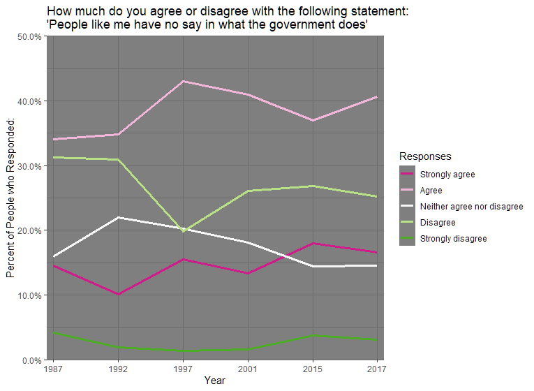
The survey_mean() command calculates the proportion of people who Strongly Agree, Agree, etc. with the statement “People like me have no say in what the government does”, and creates a new variable prop which contains these proportions. The group_by(year, nosay) command makes it so the proportions of people answering Strongly Agree etc. sum to 1 for each value of year.
And there we have it! The data is ready. All we need to do now is visualise it. I provide the code for a VERY rough and ready visualisation below. If you would like to perform your own visualisation, Healey’s book on data visualisation offers a ton of useful possibilities, and unlike for merging survey datasets, there are a lot of guides for data visualisation available via Google.
Beyond the image I also include some acknowledgements, and an Appendix where I show my work identifying the variables in different waves of the BES that I wanted to study.
9) The Result
p2 <- ggplot(data = nosaywgt, mapping = aes(x = year, y = prop,
                                            colour = nosay, group = nosay))

print(p2)

p2 + geom_line(size=1.2) +
  scale_y_continuous(labels = scales::percent,
                     expand = c(0,0),
                     breaks = seq(0,0.5,0.1),
                     limits = c(0, 0.5)) +
  scale_x_discrete(expand = c(0,0.1)) +
  theme_dark() +
  labs(title =  "How much do you agree or disagree with the following
  statement: 'People like me have no say in what the government does'",
       y = "Percent of People who Responded:",
       x = "Year",
       colour = "Responses") +
  scale_color_brewer(palette = "PiYG")
Which produces the following image:
Acknowledgements
Thank you to Chris Hanretty for advice on various syntax in this guide.
I could not have put together the string of data above, without the following guides:
“conveRt to R: the short course” by Chris Hanretty (who was also kind enough to explain the merge command to me). http://chrishanretty.co.uk/conveRt/#1
“srvyr compared to the survey package” by Greg Freedman https://cran.r-project.org/web/packages/srvyr/vignettes/srvyr-vs-survey.html
Ch.6.8 from Kieran Healey’s Data Visualisation: A Practical Introduction https://socviz.co/modeling.html#plots-from-complex-surveys
“Using the survey package in R to analyze the European Social Survey” Parts 1 & 2 by Whitt Kilburn. His blog posts were the chief inspiration for this effort. http://www.whittkilburn.org/2019/05/using-survey-package-in-r-to-analyze.html
Erik Gahner Larsen’s personal website. https://erikgahner.dk/about/
For useful advice on (i) the optimum way to organise your R projects, and (ii) how to use the here package to navigate that organisation, I recommend the following three blogs: http://jenrichmond.rbind.io/post/how-to-use-the-here-package/ by Dr Jenny Richmond https://martinctc.github.io/blog/rstudio-projects-and-working-directories-a-beginner’s-guide/ by Martin Chan https://malco.io/2018/11/05/why-should-i-use-the-here-package-when-i-m-already-using-projects/ by Malcolm Barrett
And, last but far from least, thank you to Jon Mellon and Chris Prosser for refining this blog, updating my knowledge of R, and taking the time to support this project during a plague year.
Appendix
Here I list the variables I filtered out from the datasets.
Question: “People like me have no say in what the government does”
1987
id – serialno weights – weight nosay – v109d year – year
1992
id – serialno weights – wtfactor nosay – v220b year – year
1997
id – serialno weights – wtergb nosay – govnosay year – year
2001
id – buniqidr weights – postoctw nosay – BQ65A year – year
2015
id – finalserialno weights – wt_combined_main_capped nosay – m02_3 year – year
2017
id – finalserialno weights – wt_vote nosay – m02_3 year – year